How to use SQS for disordered materials
Table of Contents
This article assumes the reader already has basic knowledge about Special Quasi-random Structure (SQS).
Preface
I am a co-author of Chapter 10: Applications of Special Quasi-random Structures to High-Entropy Alloys (M. C. Gao, C. Niu, C. Jiang, D. L. Irving) of the book High-Entropy Alloys (Ed. M. C. Gao, J. W. Yeh, P. K. Liaw, Y. Zhang, Springer, 2016). This chapter of the book focuses on the application of SQS in research with a wide variety of topics. Often, some researchers who begin to use SQS email me, asking about more basic usage of SQS. So I wrote this article, focusing on its basic usage with practical tips.
Note: the best place to seek help on the usage of mcsqs is the official ATAT forum. Dr. Axel van de Walle gave many excellent answers here.

This work is licensed under a Creative Commons Attribution-NonCommercial 4.0 International License.
Compile a mcsqs that saves all bestsqs
There is no need for me to introduce how to compile ATAT here; the manual has clear instructions. However, I have a minor complaint about how the mcsqs code handles intermediate SQS – it only saves the last one it finds as bestsqs.out. Even though this makes sense in that the last one always has the best matched correlation functions, there are other factors one needs to consider when selecting a SQS, e.g., the shape of the cell. It is better if all SQS (whether perfect or imperfect) are stored with their correlation functions. This also helps if the user uses a bestsqs for further calculations before the mcsqs finishes searching, and now there is no risk that this bestsqs gets overwritten.
To have this modified version, find the following lines in atat/src/mcsqs.c++ before compilation:
// Line 425 of mcsqs.c++
int tic=0;
Real obj=best.obj;
best.obj=MAXFLOAT;
while (1) {
  if (obj<best.obj) {
    // cerr << "Best" << endl;
    best=mc(cc);
    ofstream strfile;
    open_numbered_file(strfile, "bestsqs",ip,".out");
    strfile.setf(ios::fixed);
    strfile.precision(sigdig);
    write_structure(best.str,ulat,site_type_list,atom_label,axes,strfile);
    ofstream corrfile;
    open_numbered_file(corrfile, "bestcorr",ip,".out");
    corrfile.setf(ios::fixed);
    corrfile.precision(sigdig);
Replace the lines above with the following lines:
int tic=0;
Real obj=best.obj;
best.obj=MAXFLOAT;
int count_cniu=1;                                       // added by cniu
while (1) {
  if (obj<best.obj) {
    // cerr << "Best" << endl;
    best=mc(cc);
    ofstream strfile;
    stringstream out_cniu;                              // added by cniu
    out_cniu << count_cniu++;                           // added by cniu
    std::string str1_cniu = "bestsqs-";                 // added by cniu
    str1_cniu += out_cniu.str();                        // added by cniu
    std::string str2_cniu = "bestcorr-";                // added by cniu
    str2_cniu += out_cniu.str();                        // added by cniu
    char *cstr1_cniu = new char[str1_cniu.length()+1];  // added by cniu
    char *cstr2_cniu = new char[str2_cniu.length()+1];  // added by cniu
    strcpy(cstr1_cniu,str1_cniu.c_str());               // added by cniu
    strcpy(cstr2_cniu,str2_cniu.c_str());               // added by cniu
    open_numbered_file(strfile,cstr1_cniu,ip,".out");   // changed by cniu
    delete [] cstr1_cniu;                               // added by cniu
    strfile.setf(ios::fixed);
    strfile.precision(sigdig);
    write_structure(best.str,ulat,site_type_list,atom_label,axes,strfile);
    ofstream corrfile;
    open_numbered_file(corrfile,cstr2_cniu,ip,".out");  // changed by cniu
    delete [] cstr2_cniu;                               // added by cniu
    corrfile.setf(ios::fixed);
    corrfile.precision(sigdig);
Then compile ATAT as usual. Now the mcsqs code will save bestsqs-1.out, bestsqs-2.out, etc. with corresponding bestcorr-1.out, bestcorr-2.out, etc.
Generate SQS
Two codes from the ATAT package are needed to generate SQS: corrdump and mcsqs.
Run corrdump
The corrdump code needs an input file called rndstr.in. So let’s first talk about this input file.
The rndstr.in file
An example for FCC random solid solution:
1 1 1 90 90 90
.0 .5 .5
.5 .0 .5
.5 .5 .0
.0 .0 .0 Ni=.25,Fe=.25,Cr=.25,Co=.25
An example for L12 with partial ordering:
1 1 1 90 90 90
1 0 0
0 1 0
0 0 1
.0 .0 .0 Cr
.0 .5 .5 Ni=.333333,Fe=.333333,Co=.333334
.5 .0 .5 Ni=.333333,Fe=.333333,Co=.333334
.5 .5 .0 Ni=.333333,Fe=.333333,Co=.333334
An example for HCP random solid solution:
1 1 1.633 90 90 60
1 0 0
0 1 0
0 0 1
.000000 .000000 .0 Ni=.25,Fe=.25,Cr=.25,Co=.25
.666667 .666667 .5 Ni=.25,Fe=.25,Cr=.25,Co=.25
An example for D0-19 with partial ordering:
1 1 1.633 90 90 60
2 0 0
0 2 0
0 0 1
0.000000 0.000000 0.0 Cr
0.000000 1.000000 0.0 Ni=.333333,Fe=.333333,Co=.333334
1.000000 0.000000 0.0 Ni=.333333,Fe=.333333,Co=.333334
1.000000 1.000000 0.0 Ni=.333333,Fe=.333333,Co=.333334
0.666667 0.666667 0.5 Cr
1.666667 0.666667 0.5 Ni=.333333,Fe=.333333,Co=.333334
0.666667 1.666667 0.5 Ni=.333333,Fe=.333333,Co=.333334
1.666667 1.666667 0.5 Ni=.333333,Fe=.333333,Co=.333334
The rndstr.in input file can be divided into three parts: a unit cell (A), a periodic cell (B), and sites (C). The first line defines a unit cell (A) in the Cartesian system by defining the lengths of three vectors, a, b, c, and the angles, alpha, beta, gamma. This line can also be substituted by three lines, which represents the unit cell with a 3x3 matrix, like in a POSCAR. The purpose of the unit cell (A) is to provide a coordinate system in which the periodic cell (B) and sites (C) can be expressed. The next three lines define the periodic cell, which is the smallest supercell that represents the periodicity of the target materials. For example, a FCC random solid solution needs a one-atom FCC primitive cell, a HCP random solid solution needs a two-atom HCP primitive cell, and a L1-2 alloy needs a four-atom FCC cell. The periodic cell is expressed with the unit cell, which means the Cartesian coordinates of the periodic cell equal the multiplication of B and A. The third part is the lattice sites with atomic concentrations. Like the periodic cell (B), the site coordinates in C are also express with the unit cell (A), which means the Cartesian coordinates of the sites equal the multiplication of C and A. The concentrations of each component are suggested not to exceed 6 significant digits. The sum of concentrations on each site must always be 1.
Because the rndstr.in file is all about geometry, it is not necessary to consider the real lattice parameters in real materials. All previous examples use 1 for lattice parameter. This will make it easier to decide the -2, -3 parameters later.
The rndstr.in file does not have anything to do with the final shape of the SQS. All it does is provide all the necessary symmetry input information. The size and shape of the final SQS is controlled by the mcsqs command.
The “-2, -3” parameters
With the rndstr.in file ready, it is now time to run the first command:
corrdump -l=rndstr.in -ro -noe -nop -clus -2=1.1
The command corrdump reads the lattice file rndstr.in, and calculates symmetries and clusters. This command usually finishes very quickly, unless a very large periodic cell is defined, in which case the output file clusters.out can become really huge and the command needs a few hours or more to finish. The most important parameter of this command is “-2”, which defines the longest distance, or cut-off, when calculating the correlation functions. For example, in the case of FCC random solid solution, whose lattice parameter is 1, the first nearest neighbor distance is 2^.5/2=0.71, the second nearest neighbor distance is 1.0, and the third nearest neighbor distance is 1.5^.5=1.2. So, the cutoff should be any value between 1.0 and 1.2 if the first two shells of nearest neighbors are to be considered for pair correlation functions. Similar to the “-2” parameter, there are “-3” and above parameters for triplet correlation functions or more.
Many beginners are not sure how to determine the -2, -3 values, or how many shells of nearest neighbors to include for the matching of correlation functions. There are no general rules that work for all. Higher cutoff -2, -3 values lead to better disorder in the final structure, but also requires much longer time for the mcsqs code to find a perfectly matched SQS. The best strategy is to start with lower cutoff values (e.g., 2 shells for pairs and ignore triplets) and increase them until a good SQS is reached. Find in the following sections about how to tell if a SQS is good.
Run mcsqs
The second command mcsqs searches SQS using a Monte Carlo algorithm with defined supercell size.
Regular search
The regular search for SQS is performed by:
mcsqs -n XX
The number of atoms in the SQS, XX, must be appropriately decided. A minimal requirement is that this number must be a multiple of the number of sites in rndstr.in while also allowing integer number of atoms for all elements. For example, a ternary equiatomic L1-2 (4 sites in rndstr.in) SQS must contain at least 12 atoms.
The command mcsqs can run indefinitely, depending on the complexity of the material and the cutoffs. Usually the cutoff should include two shells; including more is usually not necessary, because if the correlation function mismatch of the second shell is not perfect, its error will most likely dominate outsider shells. For a binary alloy, the generation of SQS takes only a few seconds. For a quinary random alloy, it may never find a perfect SQS, and one that’s “good enough” may need a few days or even a couple of weeks. Here “good enough” is really up to the user’s determination. It can mean a maximum correlation mismatch of 0.1 or 0.01.
If the revised version of mcsqs is used, a series of bestsqs-XX.out will be saved. The very last one has the best correlation mismatch, but whether it is the best option for further study is arguable. Usually a SQS which has very long lattice vectors and very small angles between lattice vectors should be avoided, because it is not a comfortable model for DFT calculations.
Search with a fixed cell with sqscell.out
It is possible to control the shape of SQS. One more file needs to be taken care with here: sqscell.out. This file can be generated by the mcsqs command. A typical sqscell.out looks like this:
2

 3 -2  4
 3 -4  2
-2  4 -3

 3  0  0
 0  3  0
-1 -2  2
The first line tells the total number of cell shapes, followed by an empty line. The next three lines defines one cell shape of the SQS. This 3x3 matrix use Cartesian coordinates, NOT expressed with the unit cell in rndstr.in.
If we know what exact cell to fix for the SQS, we can put its lattice vectors in sqscell.out, which can be used to restrict the SQS generation by adding a parameter to the mcsqs command (which overwrites the -n xx parameter):
mcsqs -rc
For example, if we want to build a 2-2-2 fcc supercell with 32 atoms, we can define the sqscell.out as:
1

2 0 0
0 2 0
0 0 2
Search for SQS with equi-length vectors
The most likely reason to control the shape of SQS is to make sure its shape is as close to a cube as possible, which allows equal K-points for DFT and less symmetry-related issues. This is different from the previous situation where the user knows what exact shape to use for the SQS. Now the cell shape is undetermined. For example, we want to generate a 36-atom quaternary equiatomic bcc SQS. It’s difficult to imagine the lattice vectors for a cells that is as close to a cube as possible. For this purpose, use the following steps:
- Run
mcsqs -n 36. Stop themcsqsprocess as soon as it generates thesqscell.outfile. - Trim the
sqscell.outfile, and leave only cell shapes which have equal lattice vector lengths. If many cells have equal lengths, only use those with the shortest lengths, because it means they are the closest to a cubic shape. - Restart
mcsqs -rc
I know, Step 2 seems a boring task, so I wrote a python code for this:
#! /usr/bin/env python
#
# This script is written for Python 2.7.13.
#
# It copies sqscell.out (generated by mcsqs) to old-sqscell.out.
# Then trim the sqscell.out to three or less cells. All cells have
# equal-length lattice vectors. If more than three cells like this
# exist in the original sqscell.out, it keeps three cells with the
# smallest vector lengths.
import numpy as np

# Read the original file
with open('sqscell.out') as f1:
    lines = f1.readlines()

# Save the original file
with open('old-sqscell.out', 'w') as f2:
    for x in lines: f2.write(x)

# Replace it with a new file with 3 cells.
# The 3 cells have the smallest and equal vector lengths
with open('sqscell.out', 'w') as f3:
    tot = int(lines[0].split()[0])  # total number of cells
    count = 0
    arr1 = np.zeros((tot, 2))
    for i in range(tot):
        arr1[i][0] = i
        a1, a2, a3 = [ float(x) for x in lines[4*i+2].split() ]
        b1, b2, b3 = [ float(x) for x in lines[4*i+3].split() ]
        c1, c2, c3 = [ float(x) for x in lines[4*i+4].split() ]
        l1 = (a1**2 + a2**2 + a3**2)**.5
        l2 = (b1**2 + b2**2 + b3**2)**.5
        l3 = (c1**2 + c2**2 + c3**2)**.5
        if l1 == l2 and l2 == l3:
            arr1[i][1] = l1
            count += 1
    arr1 = arr1[arr1[:,1].argsort()]
    if count >= 3:
        j = 0
        f3.write('3\n\n')
        for i in range(tot):
            if arr1[i][1] > 0 and j < 3:
                f3.write(lines[4*int(arr1[i][0])+2])
                f3.write(lines[4*int(arr1[i][0])+3])
                f3.write(lines[4*int(arr1[i][0])+4] + '\n')
                j += 1
    else:
        f3.write(str(count) + '\n\n')
        for i in range(tot):
            if arr1[i][1] > 0:
                f3.write(lines[4*int(arr1[i][0])+2])
                f3.write(lines[4*int(arr1[i][0])+3])
                f3.write(lines[4*int(arr1[i][0])+4] + '\n')
Put this code in the same directory for mcsqs, the run it python trim.py.
Convert SQS to POSCAR
The bestsqs.out files have similar formats as the rndstr.in file. The first three lines (A) is the previously defined unit cell. The next three lines (B) is the lattice vectors of the SQS expressed with the unit cell. All following (C) is the atomic coordinates expressed with the unit cell.
To convert this SQS output to POSCAR, first calculate the lattice vectors in POSCAR as a multiplication of B and A. Next calculate the atomic coordinates as a multiplication of C and A. Remember that the atoms in the bestsqs.out are not grouped by elements! Order them by element. Then use an experimental value of the lattice parameter for line 2 in the POSCAR. Now a POSCAR using “Cartesian” format is obtained. Finally, it is recommended to further convert the “Cartesian” POSCAR to a “Directional” POSCAR, because visualization softwares like CrystalMaker or VESTA have better behavior with the latter, and it is a very good habit to visualize the POSCAR before using it for expensive DFT calculations.
Again, this looks like another boring task, so I have a tool written in C++ for it as well. It is hosted on Github (here ).
).
FAQs
How to read the output files?
Let’s focus on the output files from mcsqs, because this is the one that gives the SQS we want with its properties. The mcsqs code generates five files (or more if you count bestsqs-2.out, bestcorr-2.out, etc.): sqscell.out, rndstrgrp.out, bestsqs.out, bestcorr.out, and mcsqs.log. The sqscell.out file has been introduced previously. The rndstrgrp.out file is just a recontruction of the rndstr.in file. Let’s focus on the last three files.
The bestsqs.out file
This is the file where the SQS is stored. Its format is similar to that of the rndstr.in file, the only difference being that every site in the bestsqs.out file is an exact atom instead of a mixture of elements. It’s easy to convert the bestsqs.out file to a POSCAR, which involves matrix multiplication and sorting on the elements. As discussed previously, there is a C++ code to do the job, which I put on Github.
The bestcorr.out file
2	0.866025	-0.027778	0.000000	-0.027778
2	0.866025	-0.013889	-0.000000	-0.013889
2	0.866025	0.000000	0.000000	0.000000
2	0.866025	0.027778	0.000000	0.027778
2	0.866025	0.000000	-0.000000	0.000000
2	0.866025	0.000000	0.000000	0.000000
2	1.000000	-0.009259	0.000000	-0.009259
2	1.000000	-0.000000	-0.000000	-0.000000
2	1.000000	-0.018519	0.000000	-0.018519
2	1.000000	-0.027778	0.000000	-0.027778
2	1.000000	0.037037	-0.000000	0.037037
2	1.000000	0.000000	0.000000	0.000000
Objective_function= -0.703988
The bestcorr.out file contains the correlation functions of the target alloy and the corresponding bestsqs.out. Shown above is an example. There are five columns followed by the last line of Objective_function. The first column indicates whether this row is for pairs, triplets, etc. In the example, only pairs are considered. The second column is the distance of the neighbors that are included in the calculation. As a tip, you can confirm whether the code included all the shells as you expect. The example file shows up to the second neighbor, indicating two nearest neighbor shells are included in the calculation. These distance values also agree with defined lattice parameters (unit 1). The third column shows the correlation function results of the correponding pairs in the SQS, while the fourth the target alloy as defined in rndstr.in. The last column is the difference between column 3 and 4. The ideal SQS is reached if all numbers in column 5 are zero.
The last line of bestcorr.out gives the objective function of this SQS. The ATAT manual gives a detailed explanation of its expression. In general, this parameter discribes how good the SQS is in a universal scale. The more negative it is, the better the SQS, unless all correlation functions match with the target alloy, in which case the objective function says Perfect_match.
The mcsqs.log file
The mcsqs.log file doesn’t contain any new information. It saves the objective function and all the number in column 5 of bestcorr.out for every SQS the code finds. It is a good place to overview the calculation, as all the essential results are in this file.
How to tell if a SQS is good?
Even though the bestcorr.out file gives exact evaluation of how good the SQS is, telling whether the SQS is really good enough for the study is a more complicated problem. We can tell that a SQS with an objective function of -0.95 is better than one with that of -0.85. But it is possible the former takes 3 weeks to generate, while the latter takes only 5 days, and both turn out to be good enough. It would be great if there is a clear line, after which all SQS is good enough. But this line is dependent on the specific material and the properties of interest in each study. So, instead of giving an exact value as a fake good objective function, let’s talk about how to confirm it is a good SQS.
Elements have been assigned in rndstr.in when generating a SQS, but they can be exchanged if any two elements are equivalent, that is, always having the same concentration on the same site. For example, any two elements can be exchanged in any equiatomic fcc SQS, because all elements are equivalent. The L1-2 SQS has three equivalent elements on the B-sites (Ni, Co, Fe in the previous rndstr.in). By exchanging equivalent elements in a SQS can we obtain more than one permutations of the same SQS.
A good SQS is expected to exhibit close performance among all of its permutations. The essential property is of course its total free energy. Ideally, the total free energies of all permutations of the same SQS are equal. But this almost never happens, because it’s almost never possible to obtain a SQS that has perfect correlation functions of pairs, triplets, …, with large enough cutoffs. The energy as a function of permutation fluctuates. The fluctuation can be small or large, depending on the material, the cell size and its correlation functions (the influence of the material is most significant). It is not necessary to persue a small fluctuation with much more time-consuming SQS generation, as long as the energy scattering does not impact your conclusions.
An example is Fig. 2 in one of my papers (C. Niu, et al., Spin-driven ordering of Cr in the equiatomic high entropy alloy NiFeCrCo, Appl. Phys. Lett. 106 (2015) 161906. doi:10.1063/1.4918996):
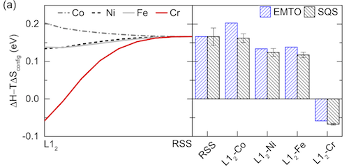
The error bars in the right figure on all SQS columns are based on all possible permutations of the same SQS. As long as these error bars don’t have an influence on the energy comparison, it is OK to have them.
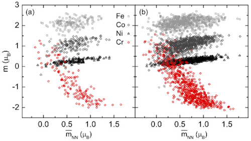
Besides total free energy, we can also use other properties to justify whether a SQS is good enough. Above is Fig. 1 in the same paper. The two subplots are from two different SQS – on the left is a small SQS with 24 atoms, and on the right is a large SQS with 120 atoms. Both SQS are for the same fcc random alloy, with similar correlation function settings. In each subplot, the magnetic moments of all atoms in all permutations are collected and plotted as a function of local neighboring magnetic environment. The right subplot has 4X more atoms, thus higher density of points. What I want to show here is that the two subplots show similar trends, which proves the accuracy of the smaller SQS. I also want to point that that this doesn’t mean a small SQS always works, but rather means it’s OK to use small SQS as long as it is proved to have good accuracy for the properties of interest.
How to accelerate the generation of SQS?
The mcsqs code does not support MPI, but runs on single CPUs. However, it supports -ip=xx to manually provide a random seed. We can submit several mcsqs instances to run independently with different random seeds. This will make it faster to find desired SQS. After all is done, select the one with the best correlation function results. Another solution is to use the -rc flag with different cell shapes for each mcsqs instance.
A mcsqs job cannot be restarted. And there is no point to restart. This is because the generation is a Monte Carlo algorithm to randomly search for structures. For example, let’s assume a running mcsqs instance at objective function = -0.8, and we want to find a SQS with an objective function = -0.9. We can continue this running job, or start with a new one. In both cases, the probability of finding the desired SQS is the same.